statistical data

statistical data

The Export and Import FOB in Romania (millions of USD)

Table 1.

Source: www.insse.ro

Requirement 1

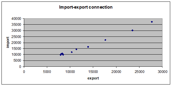
Make a graphic representation of the connection between the two variables and comment upon the scatter plot.

The chart below depicts the connection between the two variables, the imports and the exports. There is an obvious general upward trend, so the relationship is clearly a positive one

Chart 1. The import-export connection

Source: www.insse.ro

Requirement 2

Estimate and comment the parameters of the regression function, which expresses the relationship between the two variables.

The regression function in Excel yields an intercept of -1225.76and a slope of 1.3554, so that the relationship between the two can be written as follows:

y=-1225,76+1,3554x

The slope is positive, indicating a direct relationship between the two returns. In finance, this slope coefficient is called beta and it shows the sensitivity of a particular stock to the market risk.

Requirement 3

Characterize the dispersion domain around the regression function and calculate the coefficient of determination. What does this indicator mean?

In order to measure the quality of the regression function, the standard error is computed, according to the formula below:

In this case, the standard error is 684,73. This error is then used in order to estimate the coefficient of error, as follows:

The coefficient of error is 4,1% a low value which indicates the fact that the regression function illustrates well the relationship between the two returns.

Next, the coefficient of determination is calculated according to the formula:

The coefficient of determination is 99,41%, showing that the relationship between the two returns is quite strong.

Requirement 4

Find the coefficient or the ratio (index) of correlation, which synthetizes the intensity of the connection of the two variables.

The coefficient of correlation is given by the following formula:

In this case, the coefficient is 0.997, indicating very strong relationship between the two.

Requirement 5

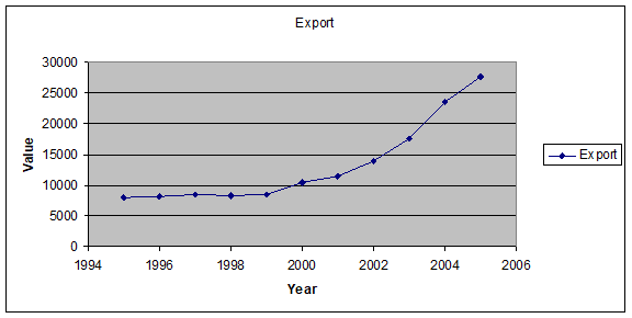
By using only one of the given series, make a graphical representation of this one and comment upon the graph.

The FOB Export in Romania

Chart 2. Evolution of Fob Exports

Source: www.insse.ro

As we can see, the values of Fob Exports regarding Romania have the tendency to increase on the term of 11 years. The 1995 values start from around eight thousand millions us dollars and we find the export values in 2005 at around 30 thousand. Until the year 2000 we have almost no fluctuation regarding exports, but after 2000 the values start rising.

Requirement 6

Determine the absolute, relative and average indicators for characterizing the variation in time of the variable that you study.

The absolute indicators :

The relative indicators are the index numbers, the percentage of change and the absolute value of a percentage change. Each of them can be calculated using a fixed or a chained base, as follows:

The average indicators are the average level, the average absolute change, the average index number and the average percentage of change. They are calculated as follows:

The situation of exports of each year can be characterized comparing the export level, as comparing the level from the year before.

For example we can state about the exports of Romanian firms in the year 2000 that they represent about 2.457 millions USD more than exports of the year 1995. Meanwhile, the exports of the year 2000 are with 2.491 millions USD over the level from the year before.

The medium annual exports specific for the period 1995-2005 is of approximately 13.243 millions USD but the indicator has no analytical value.

The exports have grown in 1995-2005, annually about 1,13 times regarding at the specific level of 1995.

We can conclude that Romania's exports are rising with about 13% annually, in the analyzedperiod.

Requirement 7

Make the analytical adjustment of the chronological series and comment upon the parameters of the analytical adjustment function.

Table 2.

Source: www.insse.ro

The parameters of the time series regression are computed according to the formulas:

The value for a=13.243,18 and b=1,839,19

The slope is positive, showing an that the adjusted exports  tended to increase from one year to another . This explains some of the positive results in the analyzed period.

Requirement 8

Characterize the residual variation according to the analytical adjustment function.

The function describes the evolution of Exports in Romania with an error of 22,66%

The error is too high to accept this result as an evolving tendency of the analyzed data.

Requirement 9

On the basis of the results obtained at points (8) and (9) estimate the probable levels of the variable in the next two months, accepting the hypothesis of a constant influence of determining factors in the studied period

For estimating the probable levels in the next 2 years we will use the adjustment function , receiving the results:

for 2006=24.278,32 millions USD

for 2007=26.117,51 millions USD